Computing for Scientists

Exercises: Lecture 1

1. Your favorites:
   • What is your favorite mathematical fact?
   • What is your favorite computational trick?
   • What is your favorite scientific problem?
   
   
2. Computers in Science: Investigate the role of computers in the study of a scientific problem of your choice, e.g. the orbit of Apollo 11 to the moon, predicting paths of hurricanes, world population in 2050, human genome, etc.

References: Lecture 1

Sumerian tablet YBC7289: An ancient calculation of sqrt(2):

Newton's Original paper: The reduction of affected equations

Raphson's Original paper: Trisection of the angle

Jean-Luc Chabert et al., A history of Algorithms, Springer-Verlag, 1994.

R.M. May (1976), "Simple mathematical models with very complicated dynamics," Nature, 261, 459-467. Review article from NATURE.

Newton's Principia :The mathematical principles of natural philosophy

The Science: Orbital Mechanics (NASA)

Hodgkin-Huxley and Fitzhugh_Nagumo Models

Deterministic Nonperiodic Flow by E. N. Lorenz, Journal of the Atmospheric Sciences, 1963; 20: 130-141.

Video Exercises References

Exercises: Lecture 2

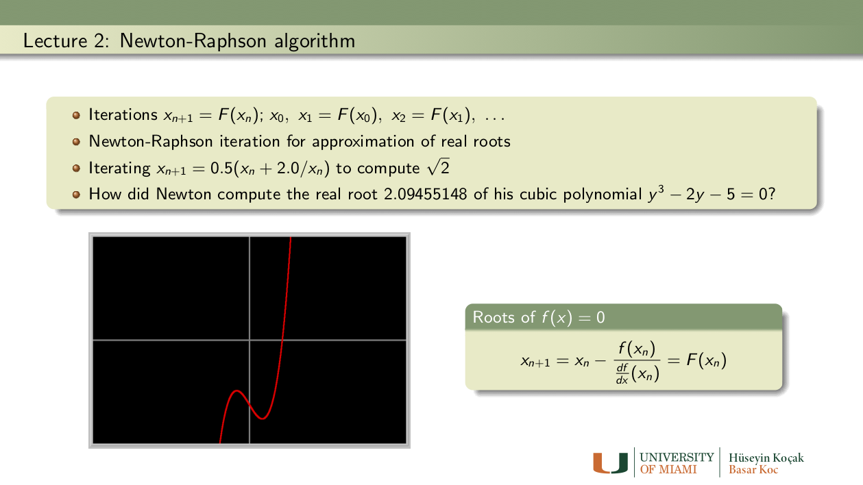
1. Newton's cubic: Using the modern version of Newton-Raphson method described in the lectures, find an approximation to a root of Newton's cubic polynomial

   y3 - 2y -5 = 0 
   

   starting with the initial guess y_0 = 2.0. To to this problem, you first need to determine which function to iterate; then enter this function into Phaser as a Custom Equation (MAP).
   • How many iterations do you have to make to get Newton's finding 2.09455148? (See Newton's original paper in the References.)
   • How good is this answer as an approximate root?
   • Why do you think Newton chose the initial condition y_0 = 2.0?
   • Try the initial conditions y_0 = 1 and y_0 = 3? Are they better or worse choices?
   • Does Newton's polynomial have any other real root? (Hint: Using a function plotter, plot the graph of the cubic polynomial.)
   
   
2. Can you beat Newton? Enter the difference equation

   x1 -> x1 - 0.21*(x1*x1 - 2)
   

   into Phaser. Iterate the initial condition x0 = 2.22 and observe that it approaches to sqrt(2). Compare the rate of convergence of this method of computing sqrt(2) with that of Newton's method

   x1 -> 0.5*(x1 + 2/x1).
   

   To make a fair comparison, use the same initial condition in both iterations. How many iterations are required to get 13 correct digits of sqrt(2) in each iteration?
   
   
3. Is faster better?: Consider the map

   x1 -> 0.375*x1 + 1.5/x1 - 0.5/(x1*x1*x1).
   

   • Iterate this map (derived by Alkalsadi around 1450AD) with the starting value 2.0 until 14 digits settle down. How many iterations are required? Now, count the number of all the additions, subtractions, multiplications and divisions you have made to obtain your approximation to sqrt(2).
   • Next do the same with Newton's method using x1 -> 0.5*(x1 + 2.0/x1).
   • Which method requires fewer number of iterations?
   • Which method requires fewer number of arithmetical operations to compute sqrt(2) to the same precision?
   
   
   
4. Heron's algorithm: Read the original paper of Heron (see the link in References). Carry out one more iteration of Heron's algorithm by hand (using paper and pencil, that is). Make sure to use fractions only. What is the error bound after this second iteration? Write the precise steps in the Heron procedure to make it an algorithm that a computer can understand. Write a paragraph about the life of Heron.
   
   
5. Trouble with Newton: Using Newton's method, with starting value x = 1, try to find a root of the function

   f(x) = -x4 + 3x2 + 2.
   

   • Does the iteration converge? Can you explain what is going wrong?
   • Can you find other initial conditions that converge to a root?
   • How many (real) roots can you find?

References: Lecture 2

Heron's Original paper: Rational approximation to sqrt(720)

Newton's Original paper: The reduction of affected equations

Newton's Method from Wikipedia

Video Exercises References

Exercises: Lecture 3

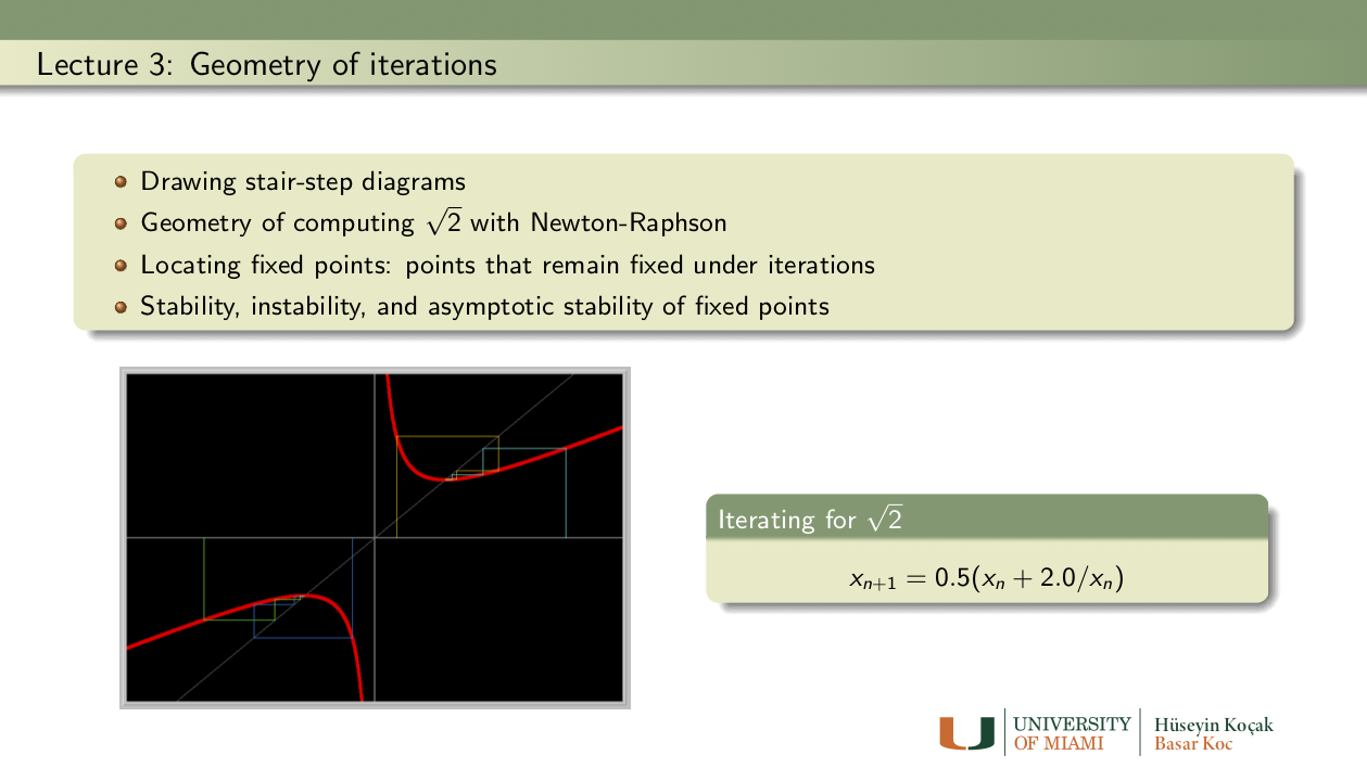
1. Real roots of Newton's cubic: Draw the stair-step diagram of the iteration for the Newton's cubic from the previous lecture. How many fixed points do you see?
   
   
2. Raphson's Cubic: Try to read the original paper of Raphson in the References. Notice that he is trying to solve the cubic equation

   3 r2 x - x3 = c r2 
   

   for the parameter values c = r = 10.0, with the initial guess of x = 3.0. Reproduce his answer for the root in Phaser using Newton-Raphson method. Draw the stair-step diagram of the iteration. How many fixed points do you see? How many real roots of Raphson's cubic are there?
   
   
3. Small angle approximation: In physics, it is often convenient to use the 'small angle approximation' by replacing sin(x) with x when x is small. Use Newton-Raphson method to find a value of x which satisfies the equation

   sin(x) - x = 0.012.
   

   How many such x can you find? Draw the stair-step diagram of the iteration process. How many fixed points do you see?
   
   
4. As a parameter is varied: Consider the map

   x1 -> a + x1 + 1.2*x1*x1 
   

   where a is a parameter. Draw at least three stair step diagrams, say, for a = -0.14, a = 0, and a = 0.14. Describe the changes in the number and stability types of fixed points as the parameter a is changed pass 0.
   
   
5. 1, 2, 3 fixed points: Consider the map

   x1 -> a + 1.6*x1 - x1*x1*x1 
   

   where a is a parameter. Find three values of the parameter a for which the map has 1, 2, or 3 fixed points. Determine the stability types of these fixed points. You should enter this map into Phaser as a Custom equation. Then using the stair-step diagrams try to find the requested parameter values. Finding a parameter value for which the map has 2 fixed points is not easy; you might have to experiment patiently.

References: Lecture 3

Raphson's Original paper: Trisection of the angle

Video Exercises References

Exercises: Lecture 4

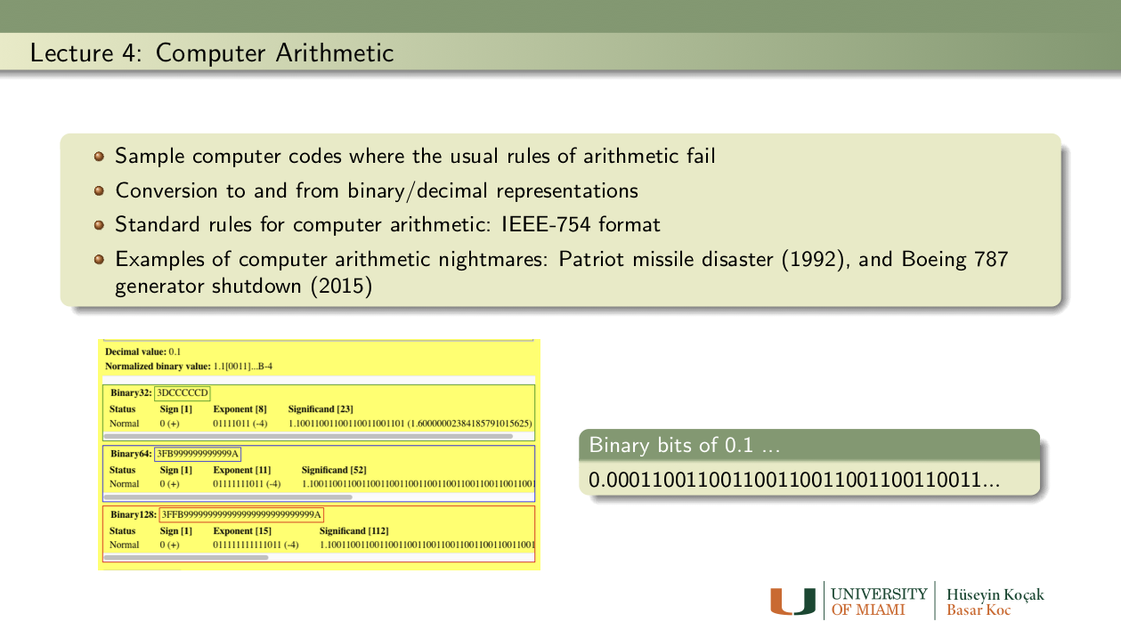
1. Binary digits: Determine the binary representation of the decimal numbers 0.1 and 9.6. Please show your computational steps.
   
   
2. Famous binary digits: Compute the first 10 binary digits of the famous numbers sqrt(2) and pi. Please show your computational steps.
   
   
3. sqrt(2) by Sumerians: On the Sumerian tablet (see the link in the References), four digits (1)(24)(51)(10) of an approximation to sqrt(2) are given in base 60. Convert this base60 approximation to base10 (decimal). Next, compute 12 binary digits of this approximation. Please show the steps of your computations. Convert this 12-bit binary number to base 10 (decimal). How many correct decimal digits of sqrt(2) do you get?
   
   
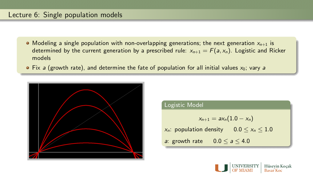
4. Logistic vs. Logistic: Arguably, one of the most famous population models is the Logistic MAP

   xn+1 = a xn (1.0 - a xn)
   

   where a is the growth rate and x_n is the density of the n-th generation. We will study this famous model in detail in future lectures.
   • Note that in the Equation -> MAP Library of Phaser, there are two versions of the logistic MAP:

     Logistic MAP: x1 -> a*x1*(1 - x1) 
     

     Logistic III MAP: x1 -> a*x1 - a*x1*x1
     

     These two maps are mathematically identical (just open up the parantheses). On the computer, however, they can behave differently.
   • Set a = 4.0 and iterate the initial condition 0.23, first using Logistic MAP and next using Logistic III MAP.
   • In the Xi Values view, look at the two sets of numbers. Do the numbers look the same at each iterate? If not, at which iterate the values have no digits in common?
   • Do you like one set of numbers better than the other?
   • What do you make of this puzzling, and disturbing, computational experiment? For a possible hint, read about the floating-point arithmetic in the References.
   
   
5. Your favorite computer trouble: Write a short report (half a page?) about your favorite, or scariest, hardware, software, security, etc. problem. Please indicate your sources.

References: Lecture 4

Sumerian tablet YBC7289: An Ancient calculation of sqrt(2)

Number Systems: Working with various bases

GOA report: Patriot disaster

Floating Point Arithmetic.

IEEE-754 Standards for Floating Point

IEEE-754 calculator

Floating Point Add/Subtract

FAA report: Boeing 787 Generator Control Unit (GCU) trouble

Video Exercises References

Exercises: Lecture 5

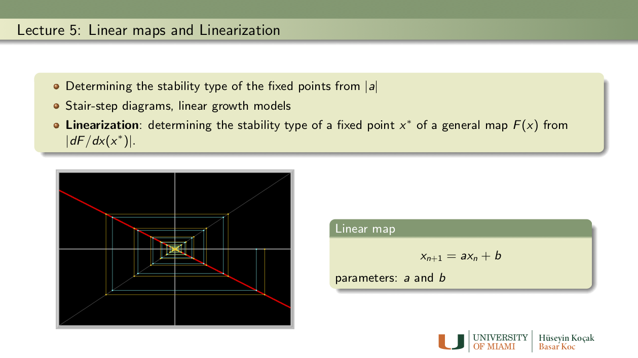
1. All linear maps: Describe the fixed points and their stability types of the linear map

   x1 -> a*x1 + b 
   

   for all values of the parameters a and b, and initial conditions x_0. Note: This equation is in the MAP library of Phaser.
   
   
2. When the Linearization does not suffice: Using Phaser, determine if the origin is an unstable or asymptotically stable fixed point of the following maps:

   1. x1 ->  x1 - 1.2*x1*x1*x1
   2. x1 ->  x1 + 1.2*x1*x1*x1
   3. x1 -> -x1 - 1.2*x1*x1*x1
   4. x1 -> -x1 + 1.2*x1*x1*x1
   

   Make sure to include one screen image of stair-step diagram for each map. Show that derivative of each equation at the origin is either 1 or -1 so that the Linearization Theorem is not useful in determining the stability type of the origin (e.g. when the derivative is 1 or -1, the stability type of the fixed point, whether is unstable or asymptotically stable, depends on the nonlinear terms of the equation).
   Hint: Enter the MAP

   x1 -> a*x1 + b*x1*x1*x1 
   

   into Phaser. Now set the parameter values appropriately to study any one of the maps above.
   
   
3. As a parameter is varied: Consider the map

   x1 -> a + x1 + 1.2*x1*x1 
   

   where a is a parameter. Draw at least three stair step diagrams, say, for a = -0.14, a = 0, and a = 0.14. Describe the changes in the number and stability types of fixed points as the parameter a is changed pass 0.
   
   
4. 1, 2, 3 fixed points: Consider the map

   x1 -> a + 1.6*x1 - x1*x1*x1 
   

   where a is a parameter. Find three values of the parameter a for which the map has 1, 2, or 3 fixed points. Determine the stability types of these fixed points. You should enter this map into Phaser as a Custom equation. Then using the stair-step diagrams try to find the requested parameter values. Finding a parameter value for which the map has 2 fixed points is not easy; you might have to experiment patiently.
   
   
5. How much can you borrow?: Suppose you borrow x₀ dollars from a bank at 2 per cent per month interest, and that you pay your bank 40 dollars per month. Derive the difference equation that models your debt to the bank at the end of each month. (Hint: the equation you need is a linear equation. So use the Linear 1D in the Map library of Phaser and set the parameters appropriately.)
   • If your original debt is 680 dollars, how long will it take you to pay the loan?
   • If your original debt is 3700 dollars, how long will it take you to pay the loan?
   • What is the maximum amount you can barrow?
   
   
6. Investing for Medical School: Suppose you want to make an investment that will pay for your child's Medical School education. You figure you will need $59,000 when your child starts Med School, 21 years from now. You can buy a long term certificate of deposite, or CD, that pays a 6.5 per cent annual interest compounded monthly. What size CD should you buy?
   Hint: Use the linear equation

   x1 -> (1.0 + 0.065/12)*x1 .
   

   To get this equation use the Linear 1D in the Map library of Phaser and set the parameters appropriately.
   
   
7. Retirement funds: Suppose you want to save 800,000 dollars over the next 30 years. To this end, suppose that you open a savings account that pays 7 percent annual simple interest. How many dollars per year should you deposit into your account to achive your goal when you retire in 30 years? Use the Linear-1D MAP in Phaser with the appropriate parameter values. It may be difficult to find the exact parameter values to have 800,000 dollar; if you have a little more money when you retire, that is fine.
   
   
8. Growing E. Coli: Suppose that a population of 320 E. Coli grows %3.1 per hour. Assuming the linear model, how many hours does it take for the population to double? How many more hours to double again? How many days to reach a population of 700,000? Does the doubling time depend on the initial population size?
   
   
9. Is faster better?: Consider the map

   x1 -> 0.375*x1 + 1.5/x1 - 0.5/(x1*x1*x1).
   

   Iterate this map (derived by Alkalsadi around 1450AD) with the starting value 1.6 until 15 digits settle down. How many iterations are required? Now, count the number of all the additions, subtractions, multiplications and divisions you have made to obtain your approximation to sqrt(2).
   Next do the same with Newton's method using

   x1 -> 0.5*(x1 + 2.0/x1).
   

   Which method requires fewer number of iterations? Which method requires fewer number of operations to compute sqrt(2) to the same precision?
   
   
10. Why Alkalsadi works: Show that sqrt(2) is a fixed point of the MAP of Alkalsadi given in the previous problem. Show that the fixed point is asymptotically stable using the Linearization Theorem. What is the value of the derivative at the fixed point?
    Extra: Can you explain why this MAP converges faster than the Newton iteration?
    
    
11. Newton's cubic again: Prove, using the Linearization theorem, that the fixed point of the map used to compute the real root of Newton's cubic

    y3 -2y -5 = 0
    

    is asymptotically stable. Hint: We have found an approximate root in an earlier week to check Newton's result. Now, take a value slightly less than the fixed point and another value greater than the fixed point. Show that derivative of the map in this interval is less than one.

References: Lecture 5

Compound interest calculater from investor.gov

Video Exercises References

Exercises: Lecture 6

1. Sensitive dependence on initial conditions: Using the Logistic model
   x_n+1 = a x_n (1.0 - x_n)
   perform the following numerical experiments:
   • Set a = 2.66. Take two initial population sizes and determine the population densities after 70 generations. Suppose that you make 0.0003 percent error in the determination of the initial population sizes. Determine the relative percentage error in the population densities after 70 generations.
   • Repeat the same experiment with the growth rate a = 3.951.
   • What are the biological implications of these experiments?
   
   
2. Logistic vs. Logistic: Note that in the Equation -> MAP Library of Phaser, there are two versions of the logistic MAP:

   Logistic MAP:     x1 -> a*x1*(1 - x1) 
   Logistic III MAP: x1 -> a*x1 - a*x1*x1
   

   These two maps are mathematically identical (just open up the parantheses). On the computer, however, they can behave differently.
   • Set a = 2.7 and compute 70 iterates of the initial condition 0.23 first using Logistic MAP and next using Logistic III MAP. In the Xi Values view, look at the two sets of numbers. Do the numbers look the same at each iterate?
   • Now set a = 4.0, compute 70 iterations of the same initial condition with both versions of the Logistic. Do the numbers look the same? If not, at what iterate the values have no digits in common?
   • What do you make of this puzzling, and disturbing, computational experiment? What are the biological implications?
   
   
3. Ricker model:

   xn+1 = xn * exp(r*(1- xn/k))
   

   This is a biologically important fisheries model containing two parameters r (growth rate) and k (carrying capacity). We assume that both parameters take on non-negative values. See the links in the References for further information on this model, including the original paper of Ricker.
   • Fix the carrying capacity at k = 1, and vary the growth rate r. Describe how the growth curve changes as r varied. Repeat the experiment for k = 1.8.
   • Fix the growth rate r = 2, and vary k. How does the growth curve depend on k?

References: Lecture 6

H. Kocak, S. Elaydi, and T. Ribble, Discrete population models and their simulations.

Ricker's original paper: W. E. Ricker, "Stock and Recruitment," Journal of the Fisheries Research Board of Canada, 1954, Vol. 11, No. 5 : pp. 559-623.

Ricker MAP: A Phaser Ecology Module

Video Exercises References

Exercises: Lecture 7

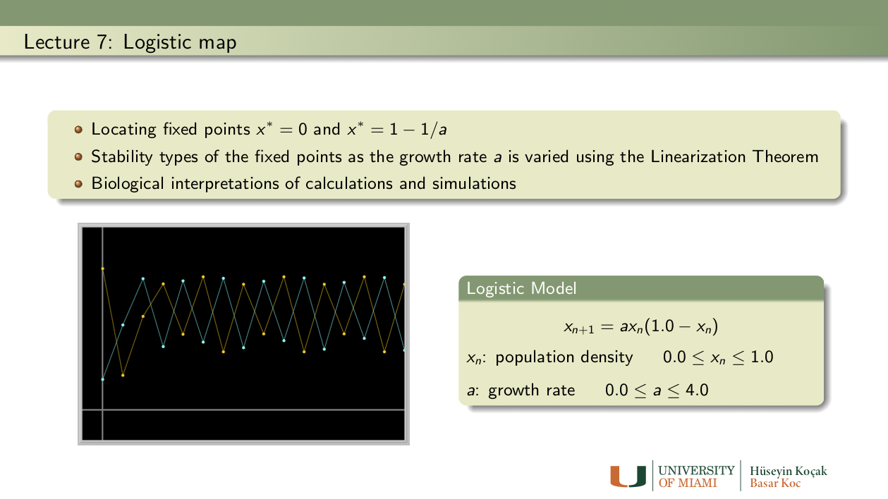
1. Fixed points of the Logistic MAP: Find all fixed points of the Logistic map

   x1 -> a*x1*(1.0 - x1)
   

   as a function of the parameter a ( answer: x = 0 and x = 1 - 1/a).
   • For which values of a these fixed points are biologically relevant?
   • Using the Linearization Theorem, determine the values of the parameter a for which the fixed point at the origin is asymptotically stable or unstable. Next do the same for the second fixed point.
   • Note that for a = 3, the positive fixed point has derivative -1 and thus the Linearization Theorem does not apply. Using PHASER determine if this fixed point is asymptotically stable or unstable for a = 3.
   
   
2. Beverton-Holt Stock-recruitment model:

   xn+1 = rxn/[1 + ((r - 1)/k)xn]
   

   This is a biologically important fisheries model containing two parameters r (growth rate) and k (carrying capacity). Despite its complicated form, this model has simple dynamics. We assume that both parameters take on positive values. Enter this model into Phaser.
   • To understand the geometric meanings of the parameters, fix k (say at 1.25) and vary r. Make a Gallery of growth curves using the stair-step view of PHASER (study the Phaser Tutorials Lesson 6 and Lesson 13 to learn about the Gallery and making SlideShow). You may want to take big window size (-1 , 15; -1, 15) to see what happens as the population gets large. Next, fix r = 1.35 and vary k. Describe biologically what you observe in these two sequences.
   • Find the fixed points of the model as a function of the parameters. For what ranges of the parameters the fixed points are biologically significant?
   • Determine the stability type of the fixed points, using the Linearization Theorem. Can the positive fixed point become unstable as the parameter r or k is increased?
   • Write a summary of the possible dynamics of a population descibed by the Beverton-Holt model and interpret your findings in biological terms.
   
   
3. A cubic map from genetics with multiple attractors: The cubic map
   

   xn+1 = (1 - a) xn + a xn3
   

   is used in population genetics involving one locus with two alleles.
   Set a = 3.2. Trying various initial conditions, find two distinct period-2 orbits. Provide the Xi-values and the stair-step diagrams of the two orbits.
   Note: Recall that in the logistic map, (almost) all initial conditions went the same attracting fixed point or periodic orbit. This is not always the case with all models, as this map demonstrates. For more information on this map, see:
   T.D. Rogers and D.C. Whitley (1983), "Chaos in the cubic mapping," Math. Modelling, 4, 9-25.

References: Lecture 7

Beverton, R.J.H., and Holt, S.J., On the Dynamics of Exploited Fish Populations, Fishery Investigations Series II Volume XIX, Ministry of Agriculture, Fisheries and Food, 1957.

Beverton-Holt model from Wikipedia

H. Kocak, S. Elaydi, and T. Ribble, Discrete population models and their simulations.

Video Exercises References

Exercises: Lecture 8

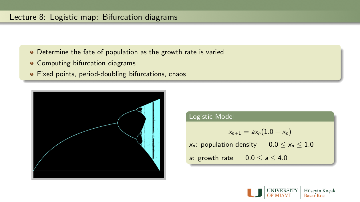
1. Period-doubling everywhere: In the Logistic MAP,

   xn+1 = a xn (1.0 - xn)
   

   set the parameter a = 3.83. Fix Start time= 1500, Stop Time=2100 and initial condition 0.208.
   • Draw the Stair-Step diagram to see the period-3 solution. Check the numbers in Xi-Values view to make sure that the numbers repeat every fourth iteration.
   • Now, change the value of the parameter a carefully to make this solution to bifurcate to a period-6 solution. Change a a bit more to obtain a period-12 solution.
   • Submit your parameter values, Xi values, and the Stair-Step diagrams.
   
   
2. Verifying calculations in the scientific literature: Read as much of the Nature review article by R.M. May linked in the References as you can. This could be difficult reading for you, but do not be discouraged. At least, do the following:
   • Draw the bifurcation diagram of the Logistic Map

     xn+1 = a xn (1.0 - xn)
     

   • Examine Table 3 on page 464 regarding the periodic orbits of the Logistic map. Try to verify the first three numbers on the 4th row: period 5(a) orbit appears for a = 3.7382 and disappears at a = 3.7411.
   • Is the claim in the paper true? Support your answer by drawing stair-step diagrams, Xi-values, for at least five parameter values: two near each boundary (for example, a=3.7381 and a=3.7383) and one inside.
   • Notice that there other parameter windows for which there are period 5 orbits. If you like, you can explore the rows 5(b) and 5(c).
   
   
3. A cubic map from genetics: The cubic map

   xn+1 = (1 - a) xn + a xn3
   

   is used in population genetics involving one locus with two alleles. Draw a bifurcation diagram of this map to identify a value of the parameter a at which the map undergoes a period-doubling bifurcation. Draw two stair-step diagrams before and after the bifurcation, and examine the Xi values, to demonstrate period-doubling. (Hint: the period-doubling bifurcations accumulate at a = 3.5980...) Reference: for more information on this map, see: T.D. Rogers and D.C. Whitley (1983), "Chaos in the cubic mapping," Math. Modelling, 4, 9-25.
   
   
4. Ricker model:

   xn+1 = xn * exp(r*(1- xn/k))
   

   This is a biologically important fisheries model containing two parameters r (growth rate) and k (carrying capacity). We assume that both parameters take on non-negative values. See the following link for further info on this model: Ricker MAP. You may also like to consult his original paper listed in the References.
   
   • Construct the bifurcation diagram of the Ricker MAP by fixing k = 1, and varying r. (see Figure 5 on the link above.)
   • By examing your bifurcation diagram, locate a value of r for which the map has a periodic orbit of period 3. Draw a stair-step diagram of your period-3 orbit. What are the values of the population size on this orbit?
   • Now increase r a little so that this period-3 solution undergoes a period-doubling bifurcation. Draw a stair-step diagram of your period-6 orbit. What are the values of the population on this orbit?
   
   
5. Bifurcation diagrams of the Beverton-Holt Stock-recruitment model:

   xn+1 = rxn/[1 + ((r - 1)/k)xn]
   

   This is a biologically important fisheries model containing two parameters r (growth rate) and k (carrying capacity). We assume that both parameters take on non-negative values. See the previous week for further information on this model.
   • Fix k = 1 , and draw the bifurcation diagram for r. To get useful picture, set initial condition to 0.3, StartTime=222, StopTime=444. Window size (0.5, 3) (-1, 3). When you fix k = 1 in the parameters panel, and assign the parameter r to be changed to the x-axis in the Bifurcation Diagram panel at the top of the tree, the current value of r is ignored and r is changed from x-min to x-max while k = 1 is held fixed.
   • Draw another bifurcation while k = 2 and r varied as above.
   • Interpret the diagrams in terms of the population's fate.
   • Next, draw three bifurcation diagrams by, fixing r = 0.7 and varying k, fixing r = 1 and varying k, fixing r =2 and varying k.
   • Interpret your bifurcation diagrams biologically.

References: Lecture 8

R.M. May (1976), "Simple mathematical models with very complicated dynamics," Nature, 261, 459-467. Review article from NATURE.

T.D. Rogers and D.C. Whitley (1983), "Chaos in the cubic mapping," Math. Modelling, 4, 9-25.

Ricker's original paper: W. E. Ricker, "Stock and Recruitment," Journal of the Fisheries Research Board of Canada, 1954, Vol. 11, No. 5 : pp. 559-623.

Ricker MAP: A Phaser Ecology Module

Video Exercises References

Exercises: Lecture 9

1. Linear maps in the plane: Consider the linear map in two variables depending on a parameter a:

   x1 -> 0.75*x1 + a*x2 
   x2 -> -a*x1 + 0.75*x2
   

   Notice that the origin is a fixed point for all values of a. Determine the parameter values for which the origin is unstable, stable, or asymptotically stable. Draw phase portraits to support your findings. Note: You can use the Linear 2D MAP in the MAP library of Phaser.
   Hint: There are two values of the parameter a for which the origin is stable.
   Optional: Can you answer the same questions for the linear map:

   x1 -> -0.75*x1 + a*x2  
   x2 -> -a*x1 - 0.75*x2
   

   What are the similarities and the differences in the dynamics of these two planar maps?
   
   
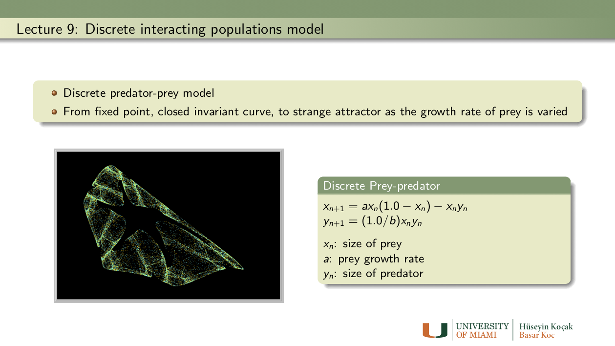
2. Bifurcation diagram for Discrete Predator-Prey: Download the following phaser Project file discrete_pp_bifurcation.ppf by just clicking on it ( or by right-click and save it to our computer. Now load this file into Phaser). You should see the following bifurcation diagram:
   
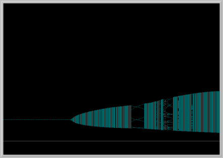
   In this diagram, parameter b is fixed and a is varied. The horizontal axis is the parameter a and the vertical axis is the x1 variable (prey). Notice that the prey population becomes periodic with period 6 in a small window of the bifurcation diagram. Pick an a value in this window and for this value of the parameter a, plot the prey and predator in the Xi vs. Time window, and also in the Phase Portrait view. Examine the numbers in Xi-Values view. Is the predator population is eventually periodic also?
   Now, do a second bifurcation diagram of x2 vs a. Do you see any differences between the two bifurcation diagrams?
   
   
3. Nicholson-Bailey model: The following pair of difference equations is a famous model that describes the intereaction of host-parasitoid populations (one insect feeds on another):
   

   Hn+1 = k Hn e( -a Pn ) 
   
   Pn+1 = c Hn [1 - e( -a Pn ) ] 
   

   
   Variables:
   H_n : Density of host at generation n
   H_n+1 : Density of host at generation n+1
   P_n : Density of parasitoid at generation n
   P_n+1 : Density of parasitoid at generation n+1
   
   Parameters:
   k : Reproductive rate of host
   a : Searching efficiency constant of parasitoid
   c : Average number of viable eggs deposited by parasitoid on a single host
   
   You can read more about this model at Phaser Web site .
   In 1941, Debach and Smith in their laboratory experiment started with 36 housefly, Musca domestica, and 18 of its pupal parasite Nasonia vitripennis and followed the populations for seven generations. They arranged the fecundity rate of the host to be 2 (k = 2, c = 1), and determined the searching efficiency constant to be a = 0.045. Please read their original paper at the link below:
   DE BACH, P. and SMITH, H.S. [1941]. "Are Population Oscillations Inherent in the Host-Parasite Relation?" Ecology, 22, 363-369. JSTOR URL
   In particular examine their data on Table I on page 367 and Figure 1 on page 368 of their article. Their Figure 1 looks like the following Phaser view: Download the following phaser Project file debach_smith.ppf by just clicking on it (or by right-click and save it to our computer. Now load this file into Phaser).
   
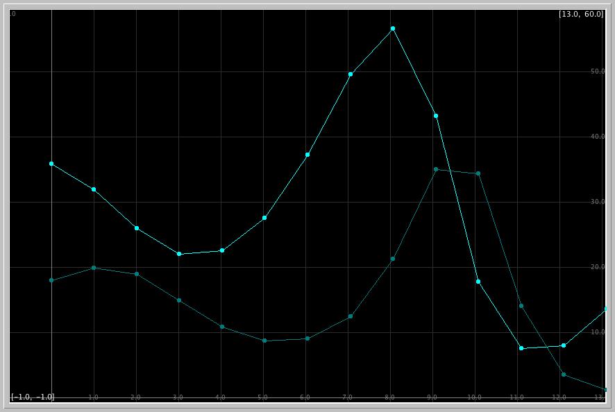
   What are the experimental counts of the host and parasitoid in the fourth and fifth generations in the paper of DeBach and Smith?
   What does the Phaser simulation of the Nicholson-Bailey model predict for these counts?
   What are the relative errors in the model predictions?

References: Lecture 9

Nicholson, A.J. and Bailey, V.A. (1935). "The balance of animal populations," Proceedings of the Zoological Society of London, 1, 551-598.

De Bach, P. and Smith, H.S. (1941). "Are Population Oscillations Inherent in the Host-Parasite Relation?" Ecology, 22, 363-369. JSTOR URL

Video Exercises References

Exercises: Lecture 10

1. Radioisotopes used in nuclear medicine: Investiagate which radioisotopes are used in nuclear medicine. Select one used in Positron Emission Tomography (PET) imaging, and another one in radiotheraphy for cancer treatment. Look up their half-lives. Use Phaser and the ODE x1' = k*x1, determine the decay constants k of the two radioisotopes you have selected. Use at least two initial conditions for each to make sure that k does not depend on the initial amount. Here is a link to get you started on radioisotopes in nuclear medicine.
   
   
2. C-14 dating: The half life of radiactive carbon C-14 is known to be appproximately 5730 years. Using Phaser, determine the decay constant k of C-14.
   
   
3. Shroud of Turin: In 1989, fibres from the Shroud of Turin were found to contain about 92% of the level of C-14 in living matter. Determine the age of the shroud using PHASER. Suppose that there was 0.3% error in the determination of the percentage of C-14 in the sample of the Shroud. What is the range of possible dates for the sample?
   Some people do not agree with the results of the C-14 dating of the Shroud. Do some research on the Web (see the links in the References, for example) and identify an objection or raise one of your own. Argue for or against the objection.
   
   
4. Libby's Nobel Lecture: Read the Nobel lecture of Willard F. Libby (Chemistry Prize in 1960) linked in the References. Why was he awarded the Nobel prize?

References: Lecture 10

W. Libby's Nobel lecture on C-14 dating

Radiocarbon dating from Wikipedia

Shroud of Turin

Radiocarbon Dating of the Shroud of Turin, by P.E Damon et al., Nature, Vol.337 (1989), pp. 611-615.

Video Exercises References

Exercises: Lecture 11

1. Computing e: Read Tutorial 1 in PHASER for computing e using the initial-value problem x' = x, x(0) = 1. Recall that the exact solution of the initial-value problem x' = x, x(0) = x₀ is x(t) = x₀ e^t. Using the method in this tutorial, compute sqrt(e), 3.4*sqrt(e), 4.4e^2, and -1/e. Check your numbers against a calculator. Report any differences. (Hints: stop your computations at the appropriate time; you can solve for negative time; you can change the initial condition.)
   
   
2. Can you have two? Consider the initial-value problem

   x' = sqrt(x),   x(0) = 0. 
   

   • Verify that the functions x(t) = 0 and x(t) = t²/4 both are solutions of the initial-value problem. Therefore, this problem does not have a unique solution.
   • Does this example invalidate the Existence and Uniqueness Theorem?
   • Try to solve this initial-value problem in Phaser. Which solution does Phaser find?
   
   
3. Race to the equilibrium: The origin (x = 0) is an asymptotically stable equilibrium point (why?) of the differential equations

   x1' = -x1,       x1' = -1.1*x1*x1*x1.
   

   • You can use the Cubic 1D ODE in the ODE library of Phaser to simulate these ODEs by setting the appropriate parameter values.
   • For which differential equation solutions approach the origin faster? First, use the initial condition x(0) = 1 for both ODEs and plot the solutions in the Xi_vs_Time view without clearing it.
   • Does your observation of speeds hold for other initial conditions? Try at least one other initial condition.

References: Lecture 11

Ordinary Differential Equations (ODE) from Wikipedia

Video Exercises References

Exercises: Lecture 12

1. Bacterial growth experiment: A culture of 8 bacteria are placed in a test tube, and their numbers is counted daily. At first, when their numbers was small they grew at a rate of %185 per day. After a few days, their numbers stabilized at about 410.
   • We will assume that the bacteria grow according to the logistic model

     x'= ax - bx2. 
     

     Find the equilibrium points of this differential equation. Assuming that a>0 and b>0, determine the stability types of the equilibria using the linearization theorem.
   • Determine the numerical values of the parameters a and b for our bacterial growth. Hint: It is reasonable to assume that when their numbers is small, bacteria can grow "exponentially;" that is a = 1.85 is a good approximation. Now using the information about the equilibria, find b.
   • With the parameter values from above, using Phaser, determine how long it takes for the bacteria culture to grow to within %10 of the carrying capacity.
   
   
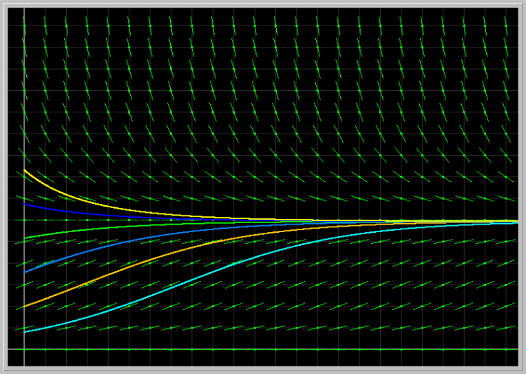
2. Another form of Logistic: Consider the continuous anolog of the logistic model using the ODE:

   x' = r x (1 - x/k)
   

   where x(t) is the population size at time t, r (growth rate) and k (carrying capacity) are positive parameters. This form of the Logistic ODE is preferred by ecologists. For r = 1 and k = 1.5, several solutions of this equation with various initial conditions are displayed in the picture below. Describe what happens to the population as the initial population size varies.
   Download the following phaser Project file logisticODE.ppf by just clicking on it (or by right-click and save it to our computer. Now load this file into Phaser). You should see the following XivsTime view:
   
   • Fix the parameter r = 1 and vary the parameter k from 0.5 to 3.0.
   • Next fix k = 1.5 and vary r from 0.5 to 4.0.
   • Describe the results of your experiments from the biological viewpoint.
   • Hint: You can use the Gallery feature of Phaser to create a sequence of pictures and animate them.
   
   
3. Another form of Logistic, cont.: Consider the continuous analog of the logistic model using the ODE:

   x' = r x (1 - x/k)
   

   where x(t) is the population size at time t, r (growth rate) and k (carrying capacity) are positive parameters.
   • Find the equilibrium points and determine their stability types for all possible parameter values using the Linearization Theorem.
   • Describe what happens to the population depending on the initial population size.
   
   
4. Proportional harvesting: Suppose that a population grows according to the logistic model, but is harvested at a rate proportional to the size of the population. The differential equation

   x' = 1.25 x - 0.16 x2 - h x 
   

   models such a population where h is the harvesting constant. Use Phaser's XivsTime view with default Algorithm Dormand-Prince 5(4) and the step size 0.01. Show that
   • If h > 1.25, then, regardless of initial population size, such a population tends towards extinction. Try several such h values and several initial conditions.
   • What happens to the population for h = 1.25 ?
   • What happens to the population if 0 < h < 1.25?
   
   
5. Harvest to extinction: Suppose that the size x(t) of a population is governed by the differential equation

   x' = 1.25 x - 0.16 x2 - 0.55.
   

   This is the logistic model with constant harvesting. Using Phaser, answer the following questions. Default Algorithm Dormand-Prince 5(4) and the Step Size 0.01 are fine to use.
   • If the initial population size is x(0) = 4.1, find the time at which the population doubles.
   • If the initial population size is x(0) = 0.4, find the time at which the population is exterminated.
   • What is the minimum initial population size for which the population does not go extinct?
   
   
6. Logistic in a periodic environment: Consider the extension of the logistic model above ODE:

   x' = r(t) x (1 - x/k(t))
   

   where x(t) is the population size at time t, r(t) (growth rate) and k(t) (carrying capacity) are parameters varying periodically in time. For specificity, take r(t) = a + b sin(t) and k(t) = c + d sin(t), where a, b, c, and d are parameters to be set.
   • Enter this equation into Phaser's Custom equation library.
   • Take a = 2, b = 1, and c = 3, d = 0, so that the growth rate is periodic but the carrying capacity is constant. Explore how various initial population sizes grow.
   • Take a = 2, b = 0, and c = 3, d = 2, so that the growth rate is constant but the carrying capacity is periodic. Explore how various initial population sizes grow.
   • Take a = 2, b = 1, and c = 3, d = 2, so that both the growth rate and the carrying capacity varies periodically. Explore how various initial population sizes grow.
   • Take a = 1, b = 1.2, and c = 3, d = 2, so that the growth rate is periodic but takes on negative values (why?) and the carrying capacity is periodic. Explore how various initial population sizes grow.
   • Try a few more parameter values of your choice and write a summary of your Phaser experiments in biological terms.
   
   
7. Gompertz model of cancer growth: The differential equation

   x' = a*(exp(-b*t))*x
   

   is used to describe the growth of a tumor, where x(t) is a measure of its size (e.g. weight or number of cells), and a and b are parameters specific to a particular tumor. To get started, let us take a = 3 and b = 2, and x(0) = 5; the solution in the XivsTime view is shown in the image below.
   
   
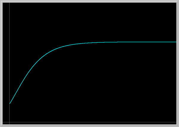
   • Load the image into your Phaser by clicking on the picture. This picture is not to scale. Adjust the Window size to get a true aspect ratio and draw the Direction Field. Using the Direction Field and solution curves answer the following questions.
   • Explain what this model predicts for the tumor growth. Experiment with several different initial tumor sizes. How does the future size of tumor depend on its initial size?
   • Experiment with several values of the parameters a and b. Explain the roles of these parameters in the tumor growth.
   • Verify, by hand, that the formula for Gompertz curve x = x_0 exp((a/b)(1 - exp(-bt))) that she gives in the article below satisfies Gompertz's differential equation above.
   • Consult the famous article "Dynamics of Tumor Growth" by A.K. Laird in British Journal of Cancer (1964) 18, 490-502. doi:10.1038/bjc.1964.55
   
   
8. Predator-Prey model: Consider the generalized predator-prey (as it appears in Phaser ODE Library)

   x1' = x1*(a - b*x2 - m*x1)
   x2' = x2*(-c + d*x1 - n*x2),
   

   where the parameters take on nonnegative values.
   • Take a = 1.5, b = 1.1, c = 1, d = 1, m = 0, n = 0, and the initial population sizes x1 = 1.5, x2 = 0.7. Determine the period and the amplitutes of the prey and predator populations.
   • Take two other sets of initial conditions of your choices and determine the periods and the amplitutes of solutions.
   • Can you locate the initial conditions which result in constant population sizes (equilibrium states)?
   • Can you make some general observations how the periods depend on initial conditions?
   
   
9. Predator-prey model with logistic growth: We considered the Predator-prey system ODE from Phaser

   x1' = x1*(a - b*x2 - m*x1) 
   x2' = x2*(-c + d*x1 -n*x2) 
   

   • Set a=2, b=1, c=1.5, d=0.5, m=0, and n=0. With these parameter values we assume that in the absence of the other, each species grows or dies exponentially.
   • Now, increase the parameter m from 0 to 3 while keeping the other parameters fixed. That is, assume that the prey grows according to the logistic model. Describe the behavior of the populations as the parameter m is varied.
   • This time, reset m = 0 and increase n from 0 to 3. What happens to the populations?
   
   
10. Epidemics: For certain infected diseases, a suceptible individual becomes infected and then either dies or recovers with immunity to the disease. Let S(t) denote the number of suceptible individuals and I(t) the number of infecteds in a population of fixed size. The change in the numbers of suceptibles and infecteds is often modeled (Kermack-McKendrick) with the pair of differential equations

    S' = -r*S*I
    I' = r*S*I - a*I
    

    where the parameters r (infection rate) and a (death or recovery rate) take on nonnegative values.
    The problem is to determine how the number of infected individuals change in time. If the number of infected individuals increase from the initial value I_0 at some some point in future time, then we say that an epidemic occurs.
    • Enter these equations into Phaser. Set a = 0.6 and r = 0.003, and the initial number of infected individuals I_0 =20. Using the Xi-Values and Xi-vs-Time views, answer the following questions.
    • If the initial number of Suceptibles S_0 is small enough, infecteds I(t) decreases from I_0 monotonically to zero --- no epidemics. If S_0 is suffciently large, the infected population first increases from I_0 to some maximum value before it dies out --- epidemics. What is the smallest number of suceptibles S_0 for which epidemics occur? This is called the threshold value for an epidemic to occur.
    • How does the treshold value depend on the parameters a and r?

References: Lecture 12

A.K. Laird, "Dynamics of Tumor Growth," British Journal of Cancer (1964) 18, 490-502. doi:10.1038/bjc.1964.55

Frank Hoppensteadt (2006) Predator-prey model. Scholarpedia, 1(10):1563.

Video Exercises References

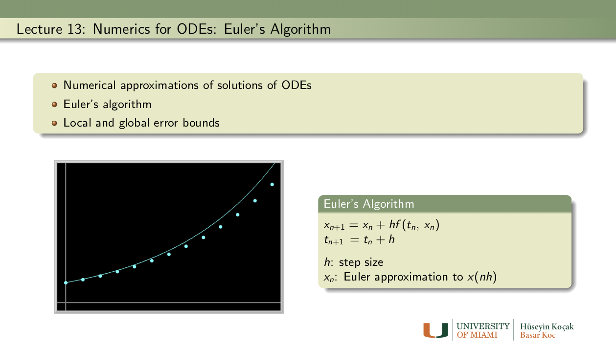
Exercises: Lecture 13

1. Euler by hand: Consider the logistic ODE:

   x' = r x (1 - x/k)
   

   where x(t) is the population size at time t, r (growth rate) and k (carrying capacity) are positive parameters. This form of the Logistic ODE is preferred by ecologists. Set r = 1.1, k = 1.6, and x(0) = 0.5, and take step size h = 0.01. By hand, compute two steps of Euler iteration. Compare the results of your hand computations with the ones you get from PHASER.
   
   
2. Error vs. step size in Euler: We showed in class that the global error bound in Euler's algorithm is proportional to the step size. Now, in Phaser solve the initial-value problem

   x' = x, x(0) = 1 to compute x(1) = e = 2.7182818284590452354,
   

   using Euler's algorithm with six different step sizes. Using your favorite plotting program, plot the errors against the step sizes. Do you get a linear relationship? If yes, what is the slope (the proportionality constant)? Be careful of the scales on your graph.
   
   
3. An explosion problem: Here we consider the "explosion" problem

   x' = x2, x(0) = 1. 
   

   This simple differential equation shows up in chemical reactions where two atoms get together to form a molecule.
   • Verify that the solution of this initial-value problem is x(t) = 1/(1-t).
   • Using Euler's Algorithm with steps h = 0.1 and h = 0.001, compute x(0.99). What is the error in your computations? Hint: What is the exact value of x(0.99) = ?
   • Now in Phaser, compute x(1) with Euler using steps h = 0.1 and h = 0.001. What is the error in your calculations?
   
   
4. How good is the error bound? Again, consider the "explosion" problem

   x' = x2, x(0) = 1. 
   

   The solution of this initial-value problem is x(t) = 1/(1-t).
   • Set h = 0.1 and compute Euler approximation for x(0.9). Determine the actual error in this approximation.
   • Recall that in the lectures we showed that for Euler

     Global error ≤ 0.5*M*t_final*h 
     

     where M is maximum of x''(t) for t between 0 and t_final. Using the global error bound formula above, determine the the value of the theoretical error bound. How does this theoretical error bound compare to actual error?
   • Repeat the calculations above for h = 0.001. Is the theoretical error bound now more realistic bound of the actual error?
   
   
5. Largest safe step size: Consider the differential equation

   x' = -12x.
   

   • Show, using the Linearization Theorem, that x = 0 is an asymptotically stable equilibrium point.
   • Now, in the XiVsTime View of Phaser, compute several solutions starting near the equilibrium point using Dormand-Prince 5(4) with the default settings. Assume that this is a correct picture (errors are very small). Your picture should indeed show the asymptotic stability of the origin.
   • Next, in the XiVsTime View of Phaser using Euler's algorithm with various step sizes compute the same solutions above. Use a large graph point size and connect points. Determine the largest step size that results in a picture where the origin looks like an asymptotically stable point as you obtain with Dormand-Prince 5(4). Hint: h = 0.3 does not give a correct picture.
   
   
6. Nonautonomous Euler: When the right-hand-side of a differential equation contains time t explicitly, the equation is called nonautonomous. Now, consider a differential equation of the form dx/dt = f (t, x) with x(t₀) = x₀. Then Euler becomes

   xn+1 = xn + h*f(tn, xn) 
   tn+1 = tn + h.
   

   Now, in the Gompertz equation x' = a*(exp(-b*t))*x, set a = 3 and b = 2.1, and x(0) = 4.5; and take step size h = 0.2. By hand (with the help of a calculator) compute two steps of Nonutonomous Euler on Gompertz and compare your numbers to the ones you get from PHASER.
   
7. Euler for systems of ODEs: Euler's algorithm can be generalized for systems of ODEs. For example, for the pair of differential equations

   dx/dt = f (x, y)
   dy/dt = g (x, y)
   

   with initial conditions x(0) = x₀ and y(0) = y₀, Euler's algorithm with step size h becomes

   xn+1 = xn + h*f(xn, yn)
   yn+1 = yn + h*g(xn, yn)
   

   Now consider the Epidemics problem from last week. Take a = 0.6, r = 0.003, S_0 = 200, I_0 = 20, and step size h = 0.2. Compute two steps of Euler by hand. Compare your numbers with those from Phaser.
   
   
8. Euler and predator-prey model: Recall that in class we considered the predator-prey system

   x1' = ax1 - bx1 x2
   x2' = -cx2 + dx1 x2
   

   where we assume that in the absence of the other, each species grows or dies exponentially. Set a = 1.2, b = 1.5, c = 1.6, and d = 1. Take the initial conditions x1(0) = 4 and x2(0) = 2. Using step size h = 0.25, compute two steps of Euler by hand. Compare your numbers with the ones you obtain from Phaser.
   
   
9. Reading Euler: Try to read the original paper of Euler listed in the References. Is his algorithm the same as the one we derived in class? What does he have to say about errors?

References: Lecture 13

Euler's original paper on his algorithm

Commentary by D. Jardine on Euler's original paper

Wikipedia: Euler's Algorithm

Video Exercises References

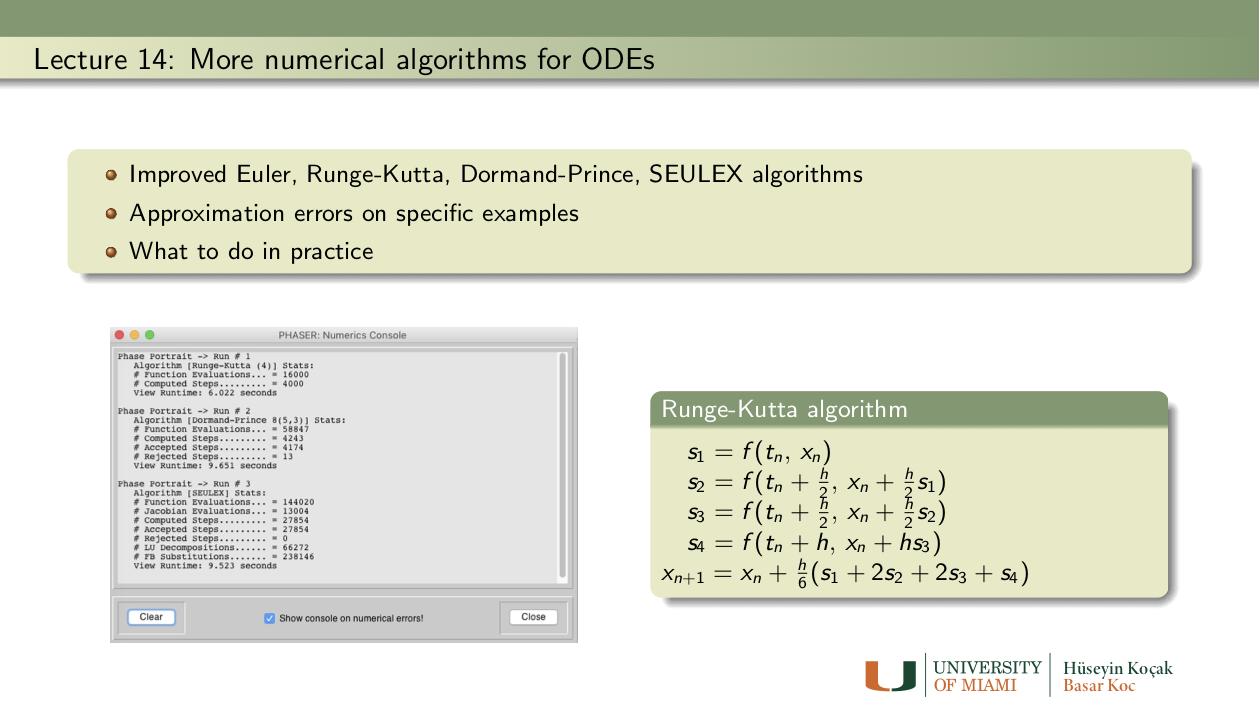
Exercises: Lecture 14

1. What to do in practice: In real life applications, it is impossible to be certain if numerically generated solutions of differential equations are reliable, or how large the errors might be. The golden rule of practice is
   • Compute the same solution using several algorithms with various step sizes and other settings.
   • If the variations in these computations are large (more than you can accept for a particular application) your problem is most likely a difficult, dangerous, or impossible one to compute.
   • If the variations in these computations are small enough, most likely you get a relatively reliable answer out of the machine.
   • Keep these recommendations in mind whenever you compute.
   
   
2. Two steps of Improved Euler(2): Consider the initial value problem

   x1' = x, x(0) = 1.
   

   With step size h = 0.5, compute, by hand using paper and pencil, two steps of Improved Euler (2) algorithm to obtain the approximate value of x(1). You can look up the formula for Improved Euler (2) in Phaser Help; make sure you show all the intermediate numbers Ks. Now compare your answer with the one you get from Phaser.
   
   
3. One step of Runge-Kutta (4): Consider our canonical example of

   x' = x, x(0) = 1.
   

   By hand, compute one step of Runge-Kutta (4) algorithm with step size of h = 1. Compare your answer to the one you obtain from Phaser. Note: The formulas for Runge-Kutta (4) are available in PhaserHelp, or in the References.
   
   
4. Orders of algorithms: Use PHASER for solving the initial-value problem

   x' = x, x(0) = 1
   

   at t = 1, that is

   x(1)= e = 2.7182818284590452354
   

   with several algorithms as follows. You should open the Console in the Numerics Editor to get the stats for your computations:
   • First use Runge-Kutta with step h = 0.01. Note that you get about 9 digits correct to the right of the decimal. How long does your computation take?
   • Now determine the "largest" step size in the Improved Euler algorithm to get the same number of correct digits. How long does it take to compute?
   • Now determine the "largest" step size in the Euler algorithm to get the same number of correct digits. How LOooooNG does it take to compute?
   • Can you explain your results in terms of the orders of the algorithms you use?
   
   
5. Impossible computation: Consider the "explosion" problem

   x' = x2,  x(0) = 1,
   

   and try to compute x(1) using several different algorithms with various step sizes.
   • Verify by differentiation that the unique solution of this initial value problem is x(t) = 1/(1-t). Conclude that x(1) is infinite.
   • Now in Phaser, compute this number, x(1), using steps h = 0.01 and h = 0.005 and algorithms Euler, Improved Euler(2), Runge-Kutta(4), Dormand-Prince5(4), and Dormand-Prince8(5,3).
   • Following "What to do in practice" rule above, conclude that this problem is indeed dangerous to compute.
   • Next, In the Dormand-Prince 5(4), set the step h = 0.01 and decrease the Absolute error and Relative error from 1.0E-7 until Phaser refuses to compute the value x(1). What is the smallest error tolerance for which PHASER refuses to compute infinity? Monitoring the Console in the Numericas Editor, report at which t value PHASER stops computations for your set tolerances.

References: Lecture 14

Runge-Kutta (4) algorithm: Read the entry in PHASER Help and also see Wikipedia: Runge-Kutta

Dormand-Prince algorithm: Read the entry in PHASER Help and also see Wikipedia: Dormand-Prince_method

Hodgkin-Huxley and Fitzhugh_Nagumo Models

Video Exercises References

Exercises: Lecture 15

1. Small angle approximation:
   
   • The Second-order differential equation given by

     x'' = (-g/l) x
     

     is the small angle approximation to the pendulum equation by replacing sin(x) with x.
   • Convert this 2nd-order ODE to a pair of first order differential equations. Enter your pair of ODEs into Phaser Custom Equation Library.
   • Set the values of g and l as you please; determine the period of oscillations for 3 initial conditions. How does the period depend on the initial conditions?
   • Set g = l = 1 and start the pendulum with 13 degrees displacement and release. Determine the period of the oscillations in the nonlinear pendulum equation (use Pendulum ODE in Phaser) and in the small angle approximation. What is the difference in the periods?
   • Set g = l = 1 and start the pendulum with 80 degrees displacement and release. Determine the period of the oscillations in the nonlinear pendulum equation and in the small angle approximation. What is the difference in the periods?
   
   
2. Lunar Pendulum:
   • In the pendulum equation in PHASER set m = 1.2, l = 1.4, and g = 1. Note that x1 is the angular position and x2 is the angular velocity of the pendulum. What is the period of the pendulum motion starting with initial angle of 1.2 radians and zero velocity? To increase the period by 12% how much do you need to change the length of the pendulum? Use the Xi vs Time view to determine the period.
   • If you take your grandfather's clock to the moon, does it slow down or speed up? By how much? (You need to look up the value of g for the moon relative to earth.)
   
   
3. A series for period:
   • There is no practical formula to compute the period of a planar pendulum without friction. However, the following infinite series
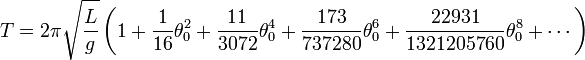
     can be used to approximate the period (with zero initial velocity) to a desired accuracy by including a finite number of the terms of the series.
   • Now take g = 1, l = 1.3, the initial angular displacement of 68 degrees (no initial velocity) and using the first 3 terms of the series compute the approximate period.
   • Compare your answer with the one you get from Phaser simuation.
   
   
4. Over the top: In the pendulum equation in Phaser set m = 1.4, l = 1.3, and g = 1. Assume that pendulum is at its stable equilibrium position. How much minimal initial velocity do you need to impart on the bob so that the pendulum goes over the top? Does this initial velocity depend on the length of the pendulum? Does it depend on the mass of the pendulum?
   
   
5. Spring-Mass System:
   
   • In Phaser ODE library use Linear Oscillation ODE for this problem. Set c = 0, f = 0, k = 1, initial conditions x1 = 1, x2 = 1. Start m = 1 and increase it to m = 9 by increments of 1. For each value of m determine the (approximate) period of the oscillations in the XiVsTime view. Now, plot these periods as a function of m using a plotting program of your choice to determine how the period depends on mass. Do you get a linear dependence?
   • Perform a similar experiment to determine the dependence of the period as function of k.
   • Resonance: Set c = 0, k = 1, m = 2, x1 = 1, x2 = 1, f = 0 and determine the period of the oscillations. Now, set f = 0.5 and determine an apprixomate value of the forcing period parameter a to set the system into resonance--unbounded oscillations. (Hint: Try to match the system period to the forcing function period.)
   
   
6. Energy conserved: The Energy of planar pendulum without friction is given by the function

   E(Θ , Θ') = (1/2)mL2(Θ')2 + mgL(1- cos(Θ)).
   

   This Energy function is supposed to be conserved along the solutions of the pendulum. Show this assertion by computing dE/dt using the chain rule, keeping in mind that Θ and Θ' depend on t, and the differential equations for pendulum. Observe that dE/dt = 0, so it must be constant function of t.
   
   
7. Free energy from EULER: Now, in the pendulum equation, take c = 0, m = 1, l = 1, g = 1, the initial conditions Θ = 0.5 and Θ'= 0 and compute the solution for 10 time units using Euler's algorithm with step size of h = 0.1. On the Time Panel of Phaser's Numerics Editor set "Skip iterations per plot" to 9 so that in the Xi Values view you will get the solution tabulated at integer values of time: you should have 11 rows of numbers. Now, use these position and velocity numbers in the formula for the Energy of the pendulum above so that you will have 11 values of the Energy function. Plot these Energy values as a function of time. Are these Energy values constant? Increasing? Decreasing?
   
   
8. Free energy from Runga-Kutta(4)? Repeat the problem above using Runga-Kutta(4), leaving all the other settings the same. Are the energy values constant? Increasing? Decreasing?
   
   
9. What did Newton say? Newton writes
   
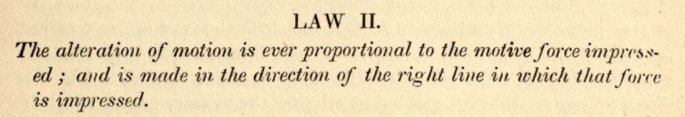
   Read his Definitions in the first several pages of his famous book Principia linked in the References. What does this original statement of LAW II have to do with

   F = ma 
   

   directly or indirectly?

References: Lecture 15

The mathematical principles of natural philosophy: Newton's Principia

Newton's Laws of Motion

Pendulum Equation

Pendulum history

Video Exercises References

Exercises: Lecture 16

1. Escape velocity: For this investigation, use the Kepler ODE in the ODE Equation Library of Phaser. Suppose that a particle of mass = 1.1 is positioned at the coordinates (2.15, 0). For this problem, first you should load the equation defaults for Kepler ODE. Then set the appropriate initial conditions to follow the shapes of the orbits.
   • Use the initial velocity components (0.0, 0.35) and admire the elliptical orbit. Double the mass to m = 2.2. Notice that the orbit gets flattened. Find the value of the vertical velocity component (0.35) that gives the previous elliptical orbit with m = 1.1.
   • Set m = 1.1 and find the minimum vertical velocity so that the particle escapes to infinity; that is, its orbit ceases to be an ellipse. You might need to use a fairly long time and a big window size to get a good estimate of the vertical escape velocity.
   • Next, double the mass of the particle. What is the new escape velocity?
   
   
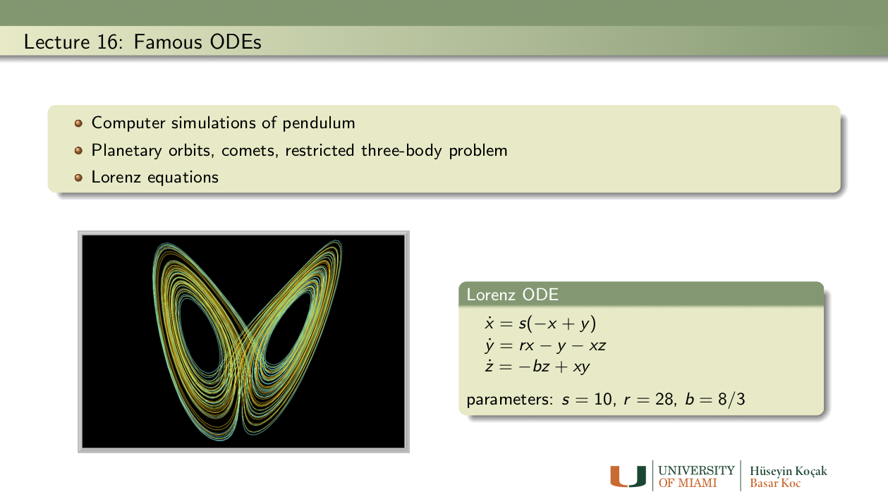
2. Onset of chaos in the Lorenz Equations: Load the Lorenz ODE in the ODE library of Phaser. Load the Equation Defaults. Set the parameter value r = 12, leave the other two parameters as they are. Notice that the two solutions approach an equilibrium value. You should be able to see this in Xi Vs. Time and Phase Portrait views. Now, increase the value of the parameter r gradually. What is the smallest value of r for which the solutions become chaotic? A chaotic solution is one that is not an equilibrium or periodic. Although there are sophisticated tests for chaotic solutions, at this point you can decide by inspection if a solution is chaotic. If necessary, you can take longer times.
   
   
3. Reading the masters: Try to read parts of the original paper Deterministic Nonperiodic Flow by E. N. Lorenz, Journal of the Atmospheric Sciences, 1963; 20: 130-141.
   • These famous differential equations (25-27) of this paper are in the ODE library of PHASER.
   • Try to reproduce some of the computational experiments descibed in the paper and create similar illustrations.
   • You should explore the three-dimensional plotting facilities of PHASER to visualize the solutions.
   
   
4. Chaos and periodicity can coexist: Unlike in the interaction of two populations, there can be chaos and more in the interaction of three or more populations. Read the original paper Chaos in Three-species food chain by Alan Hastings and Thomas Powell, Ecology, Vol. 72, No. 3 (Jun., 1991), pp. 896-903.
   • Enter the differential equations (4-5) of this paper into PHASER.
   • It is stated on page 900 that

     Also, from Fig. 4C we can deduce that for some values of b, 
     there are two separate attractors, one chaotic and one which is a limit cycle (periodic orbit). 
     This occurs both for b, lying between 2.45 and 2.48 and between 2.53 and 2.56. 
     Thus, the presence of chaotic dynamics may depend on the initial conditions, with some initial 
     conditions leading to a limit cycle, and some leading to chaos.
     

     Experiment with initial conditions to locate these two co-existing attrators.
   
   
5. Hodgkin-Huxley equations for neuron firing: A brief dicussion of the physiology of the action potential of excitable cells is presented here. Also the celebrated Hodgkin-Huxley model and its simplification due to Fitzhugh-Nagumo are introduced and their dynamics are illustrated with numerical simulations. Download the Phaser files on Hodgkin-Huxley from this site and load them into Phaser. Now determine lowest value of the input current I that causes the neuron to fire in the Hodgkin-Huxley model.

References: Lecture 16

Orbital Mechanics (NASA)

Deterministic Nonperiodic Flow by E. N. Lorenz, Journal of the Atmospheric Sciences, 1963; 20: 130-141.

Chaos in Three-species food chain by Alan Hastings and Thomas Powell, Ecology, Vol. 72, No. 3 (Jun., 1991), pp. 896-903.

Michael E. Gilpin, "Spiral Chaos in a Predator-Prey Model," The American Naturalist Vol. 113, No. 2 (Feb., 1979), pp. 306-308.

Eugene M. Izhikevich and Richard FitzHugh (2006) FitzHugh-Nagumo model. Scholarpedia, 1(9):1349.

Chaos in Ecology: Is Mother Nature a Strange Attractor? Hastings, Alan ; Hom, Carole L. ; Ellner, Stephen ; Turchin, Peter Annual Review of Ecology and Systematics, 1 January 1993, Vol.24, pp.1-33

Hodgkin-Huxley and Fitzhugh_Nagumo Models

Video Exercises References